Workers Analytics Engine offers the ability to write an extensive amount of data and retrieve it quickly, at minimal or no cost. To facilitate writing large amounts of data at a reasonable cost, Workers Analytics Engine employs weighted adaptive sampling ↗.
When utilizing sampling, you do not need every single data point to answer questions about a dataset. For a sufficiently large dataset, the necessary sample size ↗ does not depend on the size of the original population. Necessary sample size depends on the variance of your measure, the size of the subgroups you analyze, and how accurate your estimate must be.
The implication for Analytics Engine is that we can compress very large datasets into many fewer observations, yet still answer most queries with very high accuracy. This enables us to offer an analytics service that can measure very high rates of usage, with unbounded cardinality, at a low and predictable price.
At a high level, the way sampling works is:
- At write time, we sample if data points are written too quickly into one index.
- We sample again at query time if the query is too complex.
In the following sections, you will learn:
- How sampling works.
- How to read sampled data.
- How is data sampled.
- How Adaptive Bit Rate Sampling works.
- How to pick your index such that your data is sampled in a usable way.
Cloudflare's data sampling is similar to how online mapping services like Google Maps render maps at different zoom levels. When viewing satellite imagery of a whole continent, the mapping service provides appropriately sized images based on the user's screen and Internet speed.
Each pixel on the map represents a large area, such as several square kilometers. If a user tries to zoom in using a screenshot, the resulting image would be blurry. Instead, the mapping service selects higher-resolution images when a user zooms in on a specific city. The total number of pixels remains relatively constant, but each pixel now represents a smaller area, like a few square meters.
The key point is that the map's quality does not solely depend on the resolution or the area represented by each pixel. It is determined by the total number of pixels used to render the final view.
There are similarities between the how a mapping services handles resolution and Cloudflare Analytics delivers analytics using adaptive samples:
- How data is stored:
- Mapping service: Imagery stored at different resolutions.
- Cloudflare Analytics: Events stored at different sample rates.
- How data is displayed to user:
- Mapping service: The total number of pixels is ~constant for a given screen size, regardless of the area selected.
- Cloudflare Analytics: A similar number of events are read for each query, regardless of the size of the dataset or length of time selected.
- How a resolution is selected:
- Mapping service: The area represented by each pixel will depend on the size of the map being rendered. In a more zoomed out map, each pixel will represent a larger area.
- Cloudflare Analytics: The sample interval of each event in the result depends on the size of the underlying dataset and length of time selected. For a query over a large dataset or long length of time, each sampled event may stand in for many similar events.
To effectively write queries and analyze the data, it is helpful to first learn how sampled data is read in Workers Analytics Engine.
In Workers Analytics Engine, every event is recorded with the _sample_interval field. The sample interval is the inverse of the sample rate. For example, if a one percent (1%) sample rate is applied, the sample_interval will be set to 100.
Using the mapping example in simple terms, the sample interval represents the "number of unsampled data points" (kilometers or meters) that a given sampled data point (pixel) represents.
The sample interval is a property associated with each individual row stored in Workers Analytics Engine. Due to the implementation of equitable sampling, the sample interval can vary for each row. As a result, when querying the data, you need to consider the sample interval field. Simply multiplying the query result by a constant sampling factor is not sufficient.
Here are some examples of how to express some common queries over sampled data.
| Use case | Example without sampling | Example with sampling |
|---|---|---|
| Count events in a dataset | count() |
sum(_sample_interval) |
| Sum a quantity, for example, bytes | sum(bytes) |
sum(bytes * _sample_interval) |
| Average a quantity | avg(bytes) |
sum(bytes * _sample_interval) / sum(_sample_interval) |
| Compute quantiles | quantile(0.50)(bytes) |
quantileExactWeighted(0.50)(bytes, _sample_interval) |
Note that the accuracy of results is not determined by the sample interval, similar to the mapping analogy mentioned earlier. A high sample interval can still provide precise results. Instead, accuracy depends on the total number of data points queried and their distribution.
To determine the sample interval for each event, note that most analytics have some important type of subgroup that must be analyzed with accurate results. For example, you may want to analyze user usage or traffic to specific hostnames. Analytics Engine users can define these groups by populating the index field when writing an event. This allows for more targeted and precise analysis within the specified groups.
The next observation is that these index values likely have a very different number of events written to them. In fact, the usage of most web services follows a Pareto distribution ↗, meaning that the top few users will account for the vast majority of the usage. Pareto distributions are common and look like this:
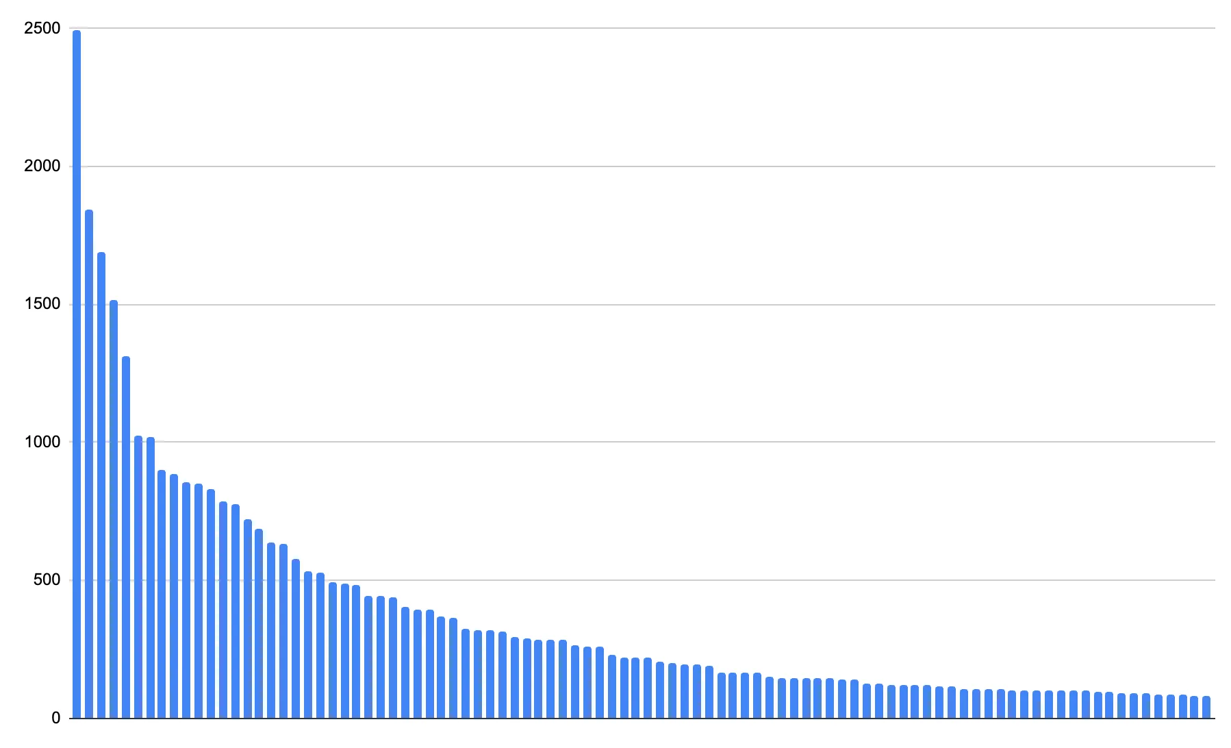
If we took a simple random sample ↗ of one percent (1%) of this data, and we applied that to the whole population, you may be able to track your largest customers accurately — but you would lose visibility into what your smaller customers are doing:
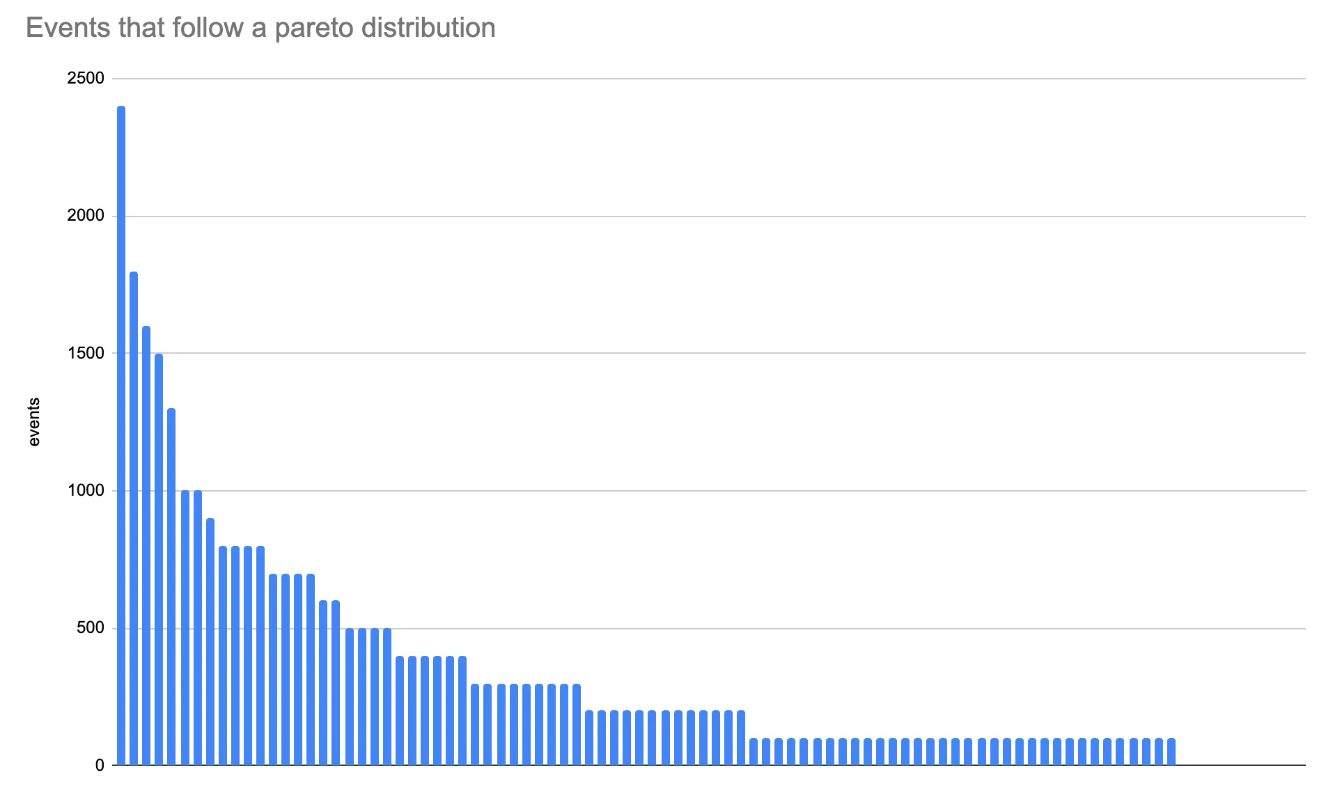
Notice that the larger bars look more or less unchanged, and yet they are still quite accurate. But as you analyze smaller customers, results get quantized ↗ and may even be rounded to 0 entirely.
This shows that while a one percent (1%) or even smaller sample of a large population may be sufficient, we may need to store a larger proportion of events for a small population to get accurate results.
We do this through a technique called equitable sampling. This means that we will equalize the number of events we store for each unique index value. For relatively uncommon index values, we may write all of the data points that we get via writeDataPoint(). But if you write lots of data points to a single index value, we will start to sample.
Here is the same distribution, but now with (a simulation of) equitable sampling applied:
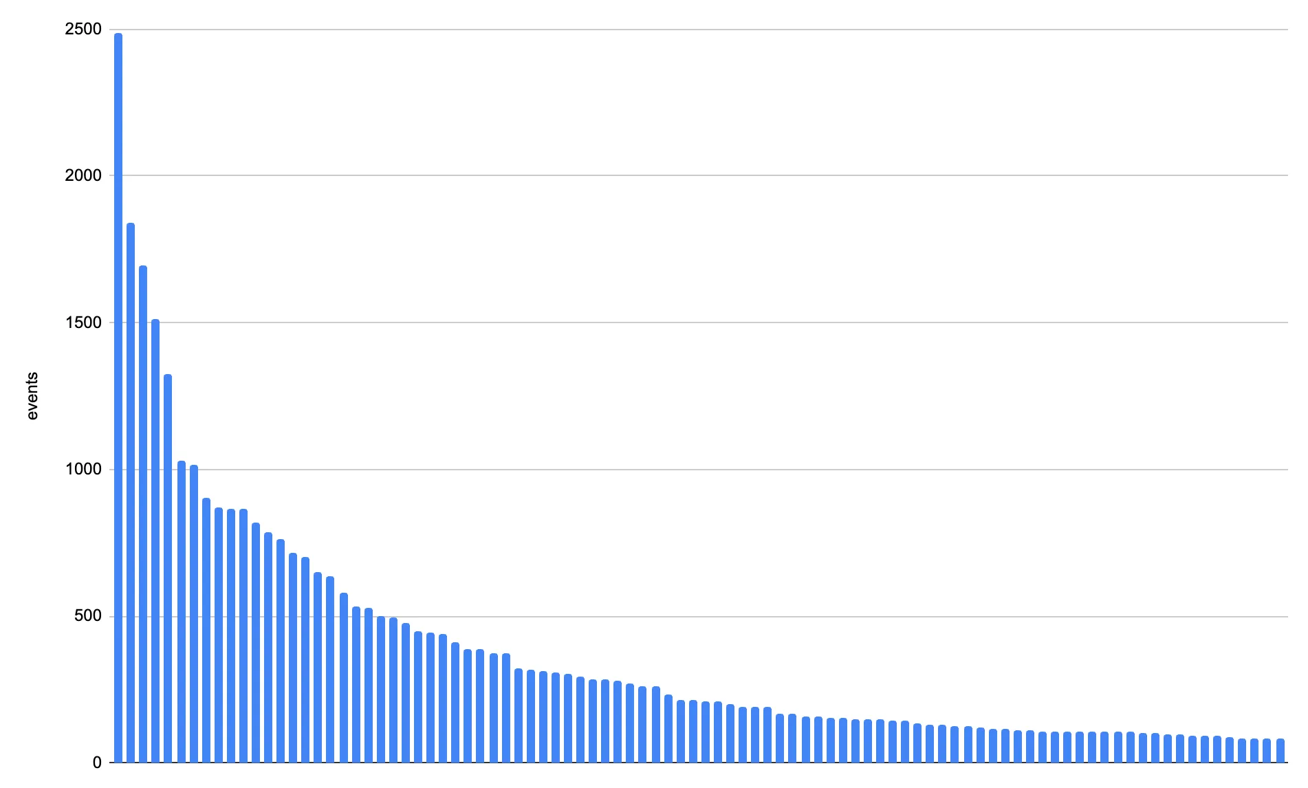
You may notice that this graphic is very similar to the first graph. However, it only requires <10% of the data to be stored overall. The sample rate is actually much lower than 10% for the larger series (that is, we store larger sample intervals), but the sample rate is higher for the smaller series.
Refer back to the mapping analogy above. Regardless of the map area shown, the total number of pixels in the map stays constant. Similarly, we always want to store a similar number of data points for each index value. However, the resolution of the map — how much area is represented by each pixel — will change based on the area being shown. Similarly here, the amount of data represented by each stored data point will vary, based on the total number of data points in the index.
Equitable sampling ensures that an equal amount of data is maintained for each index within a specific time frame. However, queries can vary significantly in the duration of time they target. Some queries may only require a 10-minute data snapshot, while others might need to analyze data spanning 10 weeks — a period which is 10,000 times longer.
To address this issue, we employ a method called adaptive bit rate ↗ (ABR). With ABR, queries that cover longer time ranges will retrieve data from a higher sample interval, allowing them to be completed within a fixed time limit. In simpler terms, just as screen size or bandwidth is a fixed resource in our mapping analogy, the time required to complete a query is also fixed. Therefore, irrespective of the volume of data involved, we need to limit the total number of rows scanned to provide an answer to the query. This helps to ensure fairness: regardless of the size of the underlying dataset being queried, we ensure that all queries receive an equivalent share of the available computing time.
To achieve this, we store the data in multiple resolutions (that is, with different levels of detail, for instance, 100%, 10%, 1%) derived from the equitably sampled data. At query time, we select the most suitable data resolution to read based on the query's complexity. The query's complexity is determined by the number of rows to be retrieved and the probability of the query completing within a specified time limit of N seconds. By dynamically selecting the appropriate resolution, we optimize the query performance and ensure it stays within the allotted time budget.
ABR offers a significant advantage by enabling us to consistently provide query results within a fixed query budget, regardless of the data size or time span involved. This sets it apart from systems that struggle with timeouts, errors, or high costs when dealing with extensive datasets.
In order to get accurate results with sampled data, select an appropriate value to use as your index. The index should match how users will query and view data. For example, if users frequently view data based on a specific device or hostname, it is recommended to incorporate those attributes into your index.
The index has the following properties, which are important to consider when choosing an index:
- Get accurate summary statistics about your entire dataset, across all index values.
- Get an accurate count of the number of unique values of your index.
- Get accurate summary statistics (for example, count, sum) within a particular index value.
- See the
Top Nvalues of specific fields that are not in your index. - Filter on most fields.
- Run other aggregations like quantiles.
Some limitations and trade-offs to consider are:
- You may not be able to get accurate unique counts of fields that are not in your index.
- For example, if you index on
hostname, you may not be able to count the number of unique URLs.
- For example, if you index on
- You may not be able to observe very rare values of fields not in the index.
- For example, a particular URL for a hostname, if you index on host and have millions of unique URLs.
- You may not be able to run accurate queries across multiple indices at once.
- For example, you may only be able to query for one host at a time (or all of them) and expect accurate results.
- There is no guarantee you can retrieve any one individual record.
- You cannot necessarily reconstruct exact sequences of events.
It is not recommended to write a unique index value on every row (like a UUID) for most use cases. While this will make it possible to retrieve individual data points very quickly, it will slow down most queries for aggregations and time series.
Refer to the Workers Analytics Engine FAQs, for common question about Sampling.